Diffusion, Entropy
and the Arrow of Time

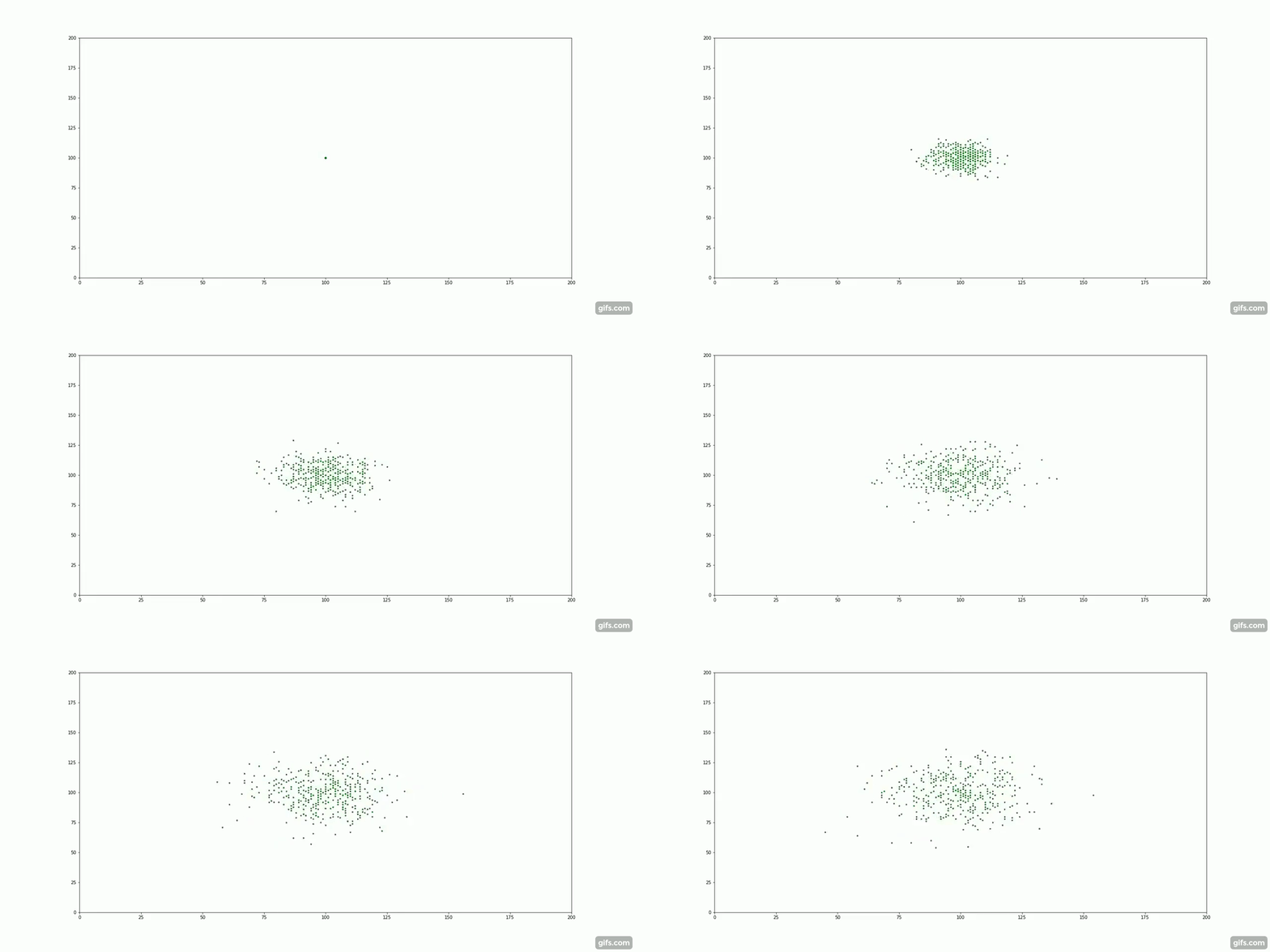
Simulating particles diffusing within a fluid.

The green particles start at the centre of the container, surrounded by an invisible "fluid".

This simulation was written in Python using the libraries "numpy" and "matplotlib".
Code for this project is available here

Explanation

Why does the world evolve? Why is it that energy spreads out and gas fills a container? The answer lies in the concept of entropy.

By analogy, entropy is a measure of the disorder of a system. It represents how "spread out" the energy has become. When you place cold cream into a hot coffee the system starts with low entropy. As heat spreads from the drink to the ice cube, the energy of the system spreads out.
The system becomes more disordered.
The entropy increases.

But how does this relate to the particle simulation above?
It turns out, particle diffusion is another example of entropy increase. Take our cream and coffee example. We first add a large dollop of cream to the coffee, all the "cream particles" clump together very closely. As time passes, the molecules of cream are subject to millions of tiny collisions with the coffee molecules. This random, molecular motion is known as Brownian Motion. With nothing but this random, repeated motion, the particles spread out to fill their container. There is no force pulling the particles away from the centre. Instead, it is the laws of probability that guide their movement.

This idea is so key to physics, that it has been summed up in its own law:

The Second Law of Thermodynamics

The entropy ( represented by S ) of a system always increases over time.

In this way, entropy "defines the arrow of time".
Entropy and time increase in the same direction.

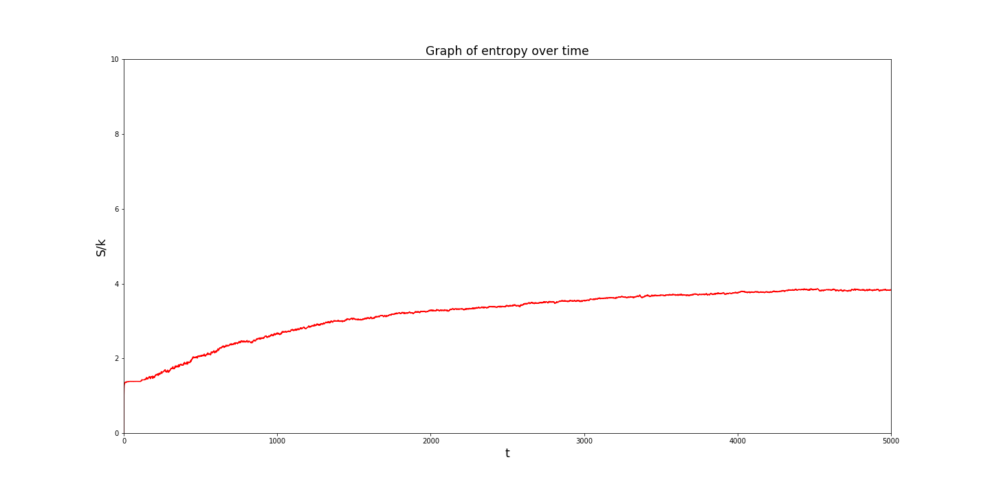
The simulation verifies the second law of thermodynamics. The programme calculates the entropy of the system at each time step.
The results are displayed below:

Side note: This is actually a graph of S/k , the entropy divided by the Boltzmann constant. Representing the entropy this way makes the numbers on the graph more manageable for a computer.

Creating the simulation

The simulation models 400 particles for 5000 time steps. In the model, the particles are all located on a "grid". This means they can only have whole number positions.
At each timestep, the particle moves in a random direction: left, right, up or down.
If a particle moves outside the 200 by 200 lattice of the simulation, then it is reflected back into the grid.
This process is repeated for each particle, for each time step.

At each step, the entropy was caculated. The simulation was divided into 64 regions. (separate to the grid sites)
The entropy was calculated using the Gibbs entropy formula:

The simulation could easily be expanded for greater lengths but the entropy increase slows as the system reaches its equilibrium.

Reference/Further Reading: Computational Physics, N.J. Giordano & H. Nakanishi, 2nd Edition